Distribution in R

There are two types of distribution in R as follow:

1. Normal Distribution
2. Binomial Distribution

Normal Distribution in R

The random collection of data from independent sources is known as normal distribution in R. Now we know that we will get a bell shape curve if we plot a graph with the value of the variable in the horizontal axis and counting the values in the vertical axis, which represent the mean of the data set. In the graph, 50% of the value is located to the left of the mean. And the rest of the 50% is to the right of the graph. This is referred to as the normal distribution.

The following functions generate normal distribution provided by R programming:

These functions can have the following parameters:

S.No	Parameter	Description
1.	x	Vector of numbers.
2.	p	Vector of probabilities.
3.	n	Vector of observations.
4.	mean	This is the mean value of the sample data whose default value is zero.
5.	sd	This is the standard deviation whose default value is 1.

dnorm():Density

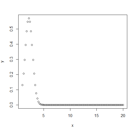
The dnorm() function is used to calculate the height of the probability distribution of each point for a given standard deviation and mean.

x <- seq(1, 20, by = .2)

# Choose the mean as 2.2 and standard deviation as 0.7.
y <- dnorm(x, mean = 2.2, sd = 0.7)

plot(x,y)

Output

pnorm():Direct Look-Up

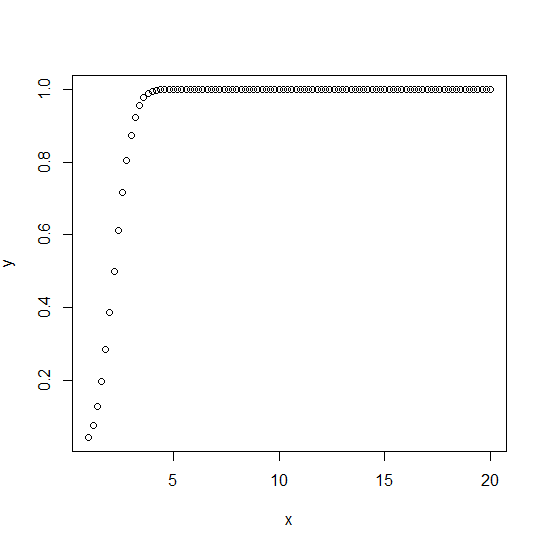
The dnorm() function is also called the “Cumulative Distribution Function”. This function calculates the probability of distributed random numbers normally, which is less than the value of a given number. Check the below cumulative distribution

f(x)=P(X≤x)

x <- seq(1, 20, by = .2)

# Choose the mean as 2.2 and standard deviation as 0.7.
y <- pnorm(x, mean = 2.2, sd = 0.7)

plot(x,y)

Output

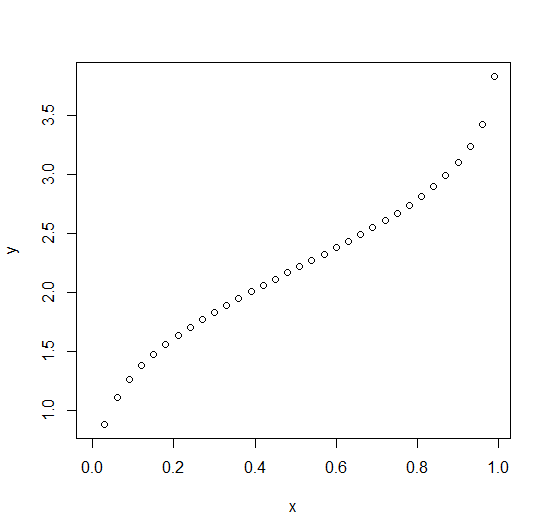
qnorm():Inverse Look-Up

The qnorm() function takes the probability value as an input and calculates a number whose cumulative values match with probability value.

p=f(x)
x=f^-1 (p)

x <- seq(0, 1, by = 0.03)

# Choose the mean as 2.2 and standard deviation as 0.7.
y <- qnorm(x, mean = 2.2, sd = 0.7)

plot(x,y)

Output

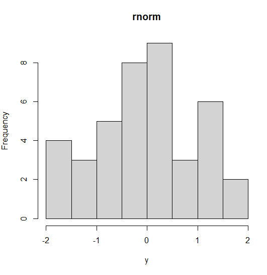
rnorm():Random variates

To generate the normally distributed random numbers rnorm() function is used.

# Create a sample of 40 numbers
y <- rnorm(40)


hist(y, main = "rnorm")

Output

Binomial Distribution in R

The binomial distribution is also called a discrete probability distribution, which is used to find the probability of success of an event. There are only two possible outcomes of events in a series of experiments. Coin tossing is the best example of the binomial distribution. At the time of toss, it gives either a head or a tail.

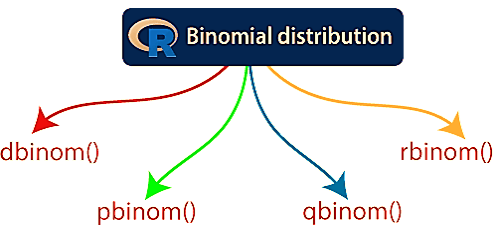
R allows us to create binomial distribution by providing the following function:

These functions can have the following parameters:

S.No	Parameter	Description
1.	x	Vector of numbers.
2.	p	Vector of probabilities.
3.	n	Vector of observations.
4.	size	This is the number of trials.
5.	prob	It is the probability of the success of each trial.

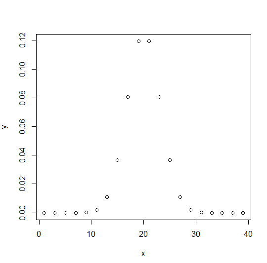
dbinom(): Direct Look-Up, Points

The dbinom() function calculates the probability density distribution at each point. In short, it calculates the density function of the specific binomial distribution.

x <- seq(1,40,by = 2)

# Create the binomial distribution.
y <- dbinom(x,40,0.5)

plot(x,y)

Output

pbinom():Direct Look-Up, Intervals

The dbinom() function of R programming calculates the cumulative probability (the single value represents the probability).  In short, it calculates the cumulative distribution function of the specific binomial distribution.

x <- pbinom(18,45,.5)

print(x)

Output

qbinom(): Inverse Look-Up

The qbinom() function of R takes the probability values and creates a number whose cumulative value match with the probability value. In short, it calculates the inverse cumulative distribution function of the binomial distribution.

x <- qbinom(0.5,45,1)

print(x)

Output

rbinom()

The rbinom() function of R programming is used to create a required number of random values for a given probability.

x <- rbinom(3,135,.5)

print(x)

Output