Nonlinear Least Square for used in regression in R. We see that it is a rare case that the equation of the model is a linear equation giving a linear graph when we used regression analysis for real-world data. Because mostly the model equation of real-world involves higher degree mathematical functions like an exponent of 3 or a sin function. Then models plot a curve instead of a line.
The aim of both linear and non-linear regression is to set model values parameters to find the line or curve that comes closest to your data. We will be able to estimate the response variable with good accuracy by finding these values.
In the least Square regression, a regression model is established in which the sum of the squares of the vertical distances of different points from the regression curve is minimized. It started from the defined model and assume some values for the coefficients. Then the nls() function is applied to get the more accurate values with the confidence intervals.
Following is the basic syntax for creating a nonlinear least square test in R:
Here:
- formula is a nonlinear model formula
- data is a data frame
- start is a named list or named numeric vector
We will the below equation to solve this problem:
Nonlinear Least Square Example
Let’s assume the initial coefficients to be 1 and 3 and fit these values into nls() function.
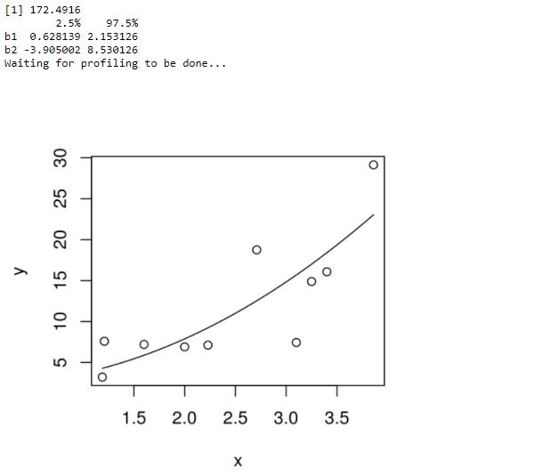
x <- c(1.6,3.1,2,2.23,2.71,3.25,3.4,3.86,1.19,1.21)
y <- c(7.19,7.43,6.9,7.11,18.75,14.88,16.06,29.12,3.21,7.58)

# Plot these values.
plot(x,y)

# Take the assumed values
m <- nls(y ~ b1*x^2+b2,start = list(b1 = 1,b2 = 3))

# Plot the chart
new.data <- data.frame(x = seq(min(x),max(x),len = 100))
lines(new.data$x,predict(m,newdata = new.data))

print(sum(resid(m)^2))

# Get the confidence intervals
print(confint(m))
Output: